K2E Canada Inc
  • Home
  • TRAINING
    • WEBINARS
    • ROAD TO EXCELLENCE ONLINE SEMINAR
    • SEMINARS
    • TECHNOLOGY CONFERENCE
    • INSTRUCTORS
  • NEWSLETTER
    • Signup
  • ABOUT
  • CONTACT
  • BLOG
  • Home
  • TRAINING
    • WEBINARS
    • ROAD TO EXCELLENCE ONLINE SEMINAR
    • SEMINARS
    • TECHNOLOGY CONFERENCE
    • INSTRUCTORS
  • NEWSLETTER
    • Signup
  • ABOUT
  • CONTACT
  • BLOG

Manage Links in Excel Workbooks

10/4/2021

 
The ability to link data from one Excel workbook to another is one of the spreadsheet application’s best features. However, managing links – including editing and deleting links – is frustrating for many users. In this article, you will learn the best ways to manage links in Excel workbooks.

Identifying And Managing Inbound Links

The most common need is to identify and manage inbound links from one or more “source” workbooks into a “destination” workbook. The need for this type of management arises from several situations, including troubleshooting calculations and auditing and verifying formulas in the destination workbook. Fortunately, there are three at least three simple ways to identify inbound links, and two of these methods facilitate editing and managing linked data with ease.

Use Excel's Find & Replace Feature To Identify Inbound Links

Perhaps the most direct method of identifying inbound links is to use Excel’s Find and Replace feature to search for all formulas containing “xlsx.” This technique works because when you link data from another workbook, the link’s text includes “xlsx.”

To utilize this technique, first open Excel’s Find and Replace dialog box using a CTRL + F keyboard sequence. Then enter “*.xlsx” in the Find what box and ensure that you enable Formulas in the Look in box as shown in Figure 1. Note that you can search for inbound links in the current worksheet only or the entire workbook. Finally, click Find All to search for all the links in the worksheet or workbook.
Picture
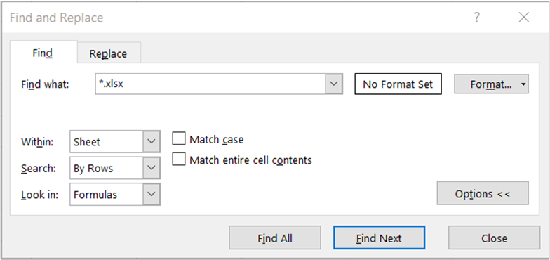
Figure 1 - Searching For Links With Excel's Find And Replace Feature

Upon executing the search, the Find and Replace dialog box displays all the links in the location searched, as shown in Figure 2. Once identified, you can manage the links – edit them or delete them – by editing the cells in which they reside.
Picture
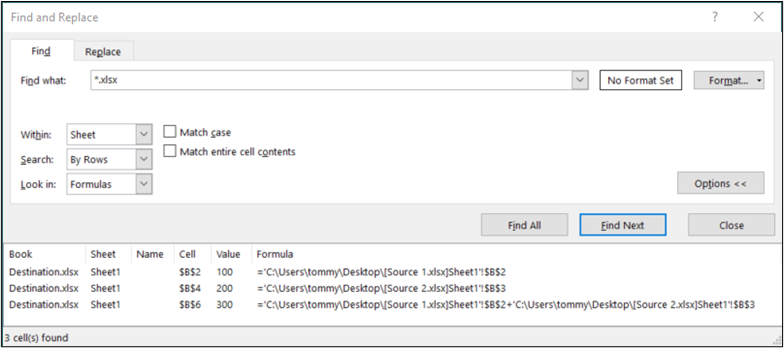
Figure 2 - Identifying Inbound Links With Find And Replace


Managing Inbound Links With Excel’s Edit Links Feature

Another option for managing inbound links in a workbook is to use Excel’s Edit Links feature. To use this feature, access it by clicking Edit Links in the Queries & Connections group on the Data tab of the Ribbon. Alternatively, you can access Edit Links by clicking File, Info, and selecting Edit Links to Files near the window’s lower right corner. Regardless of how you choose to access it, the Edit Links window appears, as shown in Figure 3. 
Picture
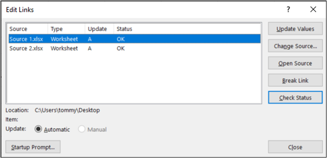
Figure 3 - Excel's Edit Links Tool

From the Edit Links window, you can choose to update the values linked into the current workbook, edit links by changing their source workbook or breaking them, open the source workbook, and check the status of a link. Note that Excel does not make these tools available if you choose the Find & Replace method of identifying links discussed previously.

Identifying Links With Excel's Inquire Add-In

A third option for identifying links to manage them is to take advantage of Excel’s Inquire add-in. Inquire is a Microsoft-provided add-in for Excel that offers tremendous capabilities for identifying risk and inconsistencies in Excel workbooks. Inquire add-in versions of Excel provided through Office Professional Plus and Microsoft 365 Apps for enterprise editions. For more information on activating Inquire, see the Microsoft-published article at https://bit.ly/3yoP2IE.

With the Inquire add-in activated, click Inquire followed by Workbook Relationship to create a Workbook Relationship report. This report, a sample of which Figure 4 displays, pictorially depicts the links from one workbook to another. Similarly, you could generate a Worksheet Relationship report to see how data flows from one worksheet to another. 
Picture
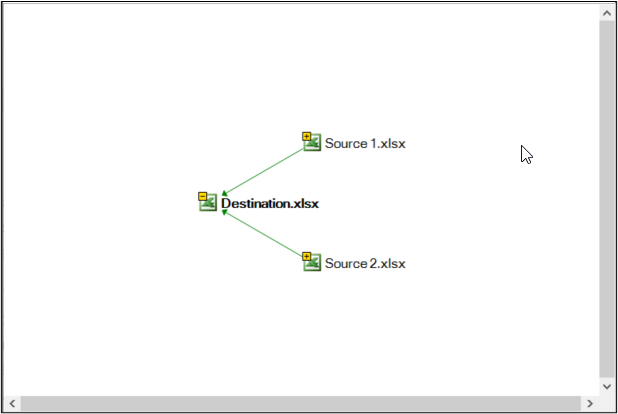
Figure 4 - Inquire's Workbook Relationship Report

For an even more detailed view of links, you can generate a Cell Relationship report that provides a granular view of all cells linking into a specific cell.
Picture
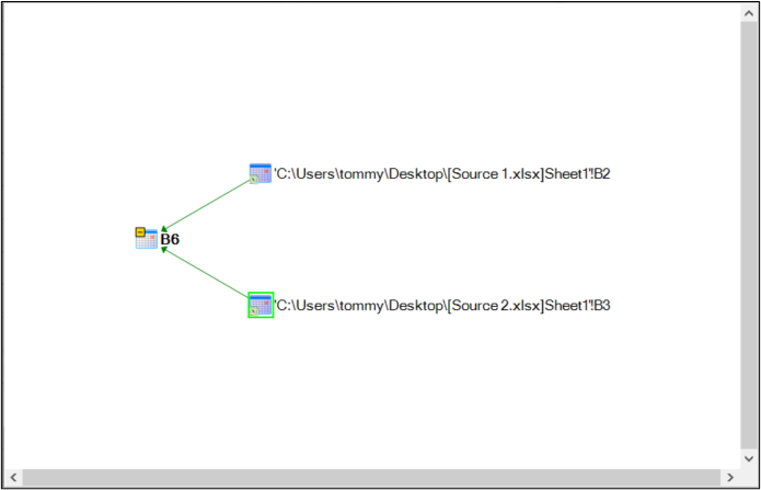
Figure 5 - Cell Relationship Report Created By Excel's Inquire Add-In

Once you identify the links with linked data, you can use any method desired to edit or deactivate the links, as necessary.

Summary

Linking data from one workbook to another is a common Excel practice. However, sometimes managing links can become unwieldy. In some cases, users end searching for linked data by inspecting each cell, one-by-one. Of course, there are better ways to manage links in Excel workbooks. For example, as outlined above, you can use Excel’s Find & Replace feature, Excel’s Edit Links tool, or the Inquire add-in to assist you in identifying linked data and managing it. So, if you need to manage links in Excel workbooks, explore the techniques discussed here to get better results in less time.
Are you interested in learning more about Excel? Consider a K2 Enterprises learning option focused on Excel. You can learn more at www.k2e.ca/training.

Tommy Stephens

Excel - My Favourite Things - Slicers

8/4/2021

 
When working with a range of related cells in Excel, my first step is to create an Excel Table. In addition to the benefits noted in my post “Excel – My Favourite Things - Excel Tables,” slicers is another feature available for Excel Tables that I often use.

Slicers are an interactive method to filter Excel Tables, PivotTables and related charts. It provides a quick way to filter data, see how it is filtered, and quickly clear the filter.

For this example, we will use a chart created from the data in an Excel Table to demonstrate the creation and configuration of a slicer.
Picture
On the Table Design tab (must have a cell within the table selected for the tab to show), click Insert Slicer. The following dialogue will open; we will select month from the list and click OK for this slicer.
Picture
Your slicer will now be an object on the Excel sheet that you can move and resize. To configure the slicer, with it selected, click on the Slicer tab on the ribbon. The Slicer tab provides configuration options, including Slicer Styles, align, and set the columns, button size, and overall size of the slicer.
Picture
One setting I find very useful under Slicer Settings is to change the Display header and check Hide items with no data.
Picture
With the slicer options completed, you can quickly filter the table and chart and clear the filter by clicking on the  icon at the top of the slicer.
Picture
Icon at the top of the slicer
Picture
Picture
Multiple slicers can be connected to the same Excel Table to allow advanced filtering.

Enjoy the simplification of filtering with Slicers in your workbooks.

Ward Blatch, CPA CA

Excel - My Favourite Things - Excel Tables

8/3/2021

 
There is rarely a workbook I use that does not contain at least one Excel Table. What is an Excel Table? An Excel Table is a range of related cells grouped to make managing and analyzing much easier. An Excel Table provides a reference to a self-expanding range of cells with a header row and filtering. In addition, an Excel Table delivers the following advantages over using just a range of cells: 

  • Excel Table name – a customizable name applied to the range of cells for easy reference and to include table cells and ranges within a formulas 
  • Excel Table formatting – providing quick and easy formatting of the data range 
  • Calculated columns – inputting a formula into a single cell will result in it being replicated to the other cells in the table column 
  • Total Row – provides a variety of calculations for a table column, including sum, count, average, and so on. 
To convert a range of related cells to an Excel Table, first make sure you have a header row (the first row containing the description of the column) and then with a cell in the range selected, click Format as Table on the Home tab.  
Picture

Clicking the command shows the Table formats available. Select the one you would like to use. Now confirm the range chosen by Excel is correct and that it has identified your first row has headers.
Picture

The range of related cells is now an Excel Table. Note the Table Design tab at the end of the ribbon. This tab is only available when you have selected a cell within the Table. The tab provides access to the Excel Table tools, including the place to change the table name, which I recommend doing.
Picture

To demonstrate one of the significant advantages of Excel Tables, we will summarize the data using the sumifs function. The sumifs function sums a range of cells based on up to 127 different criteria.
=sumifs(sum_range, criteria_range1, criteria1,….)
For our example, we will summarize the sales data by region. The Table has been renamed to Sales, and the resulting formula is as follows.
Picture

The sum range in the formula is the table name plus the column header in square brackets sales[Amount]. When typing the formula, the autocomplete will show the table name in the list of options. Then after entering the opening “[“ the list of headers is displayed in the autocomplete for selection.
Picture
Excel Tables make it much quicker and easier to input formulas correctly.

If you would like to bring your Excel skills to a new level with Excel Tables, please check out our webinar K2’s Excel Tables – Database Technology Comes to Spreadsheets – On Demand (2 hours)

Enjoy Excel Tables within your workbooks.

Ward Blatch, CPA CA

Excel Show Changes

4/5/2021

 
When co-authoring first arrived, I continued to use shared workbooks for one reason, the audit trail. Despite the significant shortcomings of shared workbooks, including my favourite feature, Excel Tables not being available.

All that has now changed.

I can finally stop using Excel Shared workbooks and enjoy the benefits of co-authoring with the introduction of Show Changes. Working on an Excel file stored in SharePoint or OneDrive with AutoSave on will now track changes. Open the file using a version that supports co-authoring; Excel app for Microsoft 365, Excel for the web or the Excel mobile apps. All your changes and everyone else that works on the file will be listed in the Changes pane.  
 
To see changes made in the past 60 days, you currently must open the Excel file using Excel for the web. From the Show Changes pane, you can change the view to be a range or sheet.
Picture
You can also right-click any cell or range and select show changes for that specific cell or range of cells.
Picture

I encourage you to check out Show Changes using the workbook on our SharePoint site, “Paper Printing & Management Analysis”.

There are, of course, some things that Show Changes does not currently track.
  • Chart, shape, and other object edits
  • Operations with PivotTable
  • Changes to formatting
  • Filtering and hiding cells or ranges and
  • Deleted location  

Some actions, including editing with a perpetual license or older version of excel, or uploading, saved copy or replaced file, will result in the changes being cleared.

Co-Authoring is now complete with Show Changes. A significant improvement to the collaboration experience. Work from any device, simultaneously with others and track the changes each person is making.

Enjoy collaborating with confidence.

Ward Blatch, CPA CA

Excel's STOCKHISTORY Function is Now Available

3/4/2021

 
Recently added to Excel is the new STOCKHISTORY function. You can use this function to retrieve historical prices for stocks as of a given date or range of dates. Read on, and you will learn how to use this feature to query historical securities prices into an Excel workbook.

Introducing STOCKHISTORY

Excel’s STOCKHISTORY function is finally rolling out to subscription-based versions of Excel. Unfortunately, this function is not yet available with perpetual licenses of Excel, such as Excel 2016 and Excel 2019. Presumptively, Microsoft will add the function to the next new version of Excel.

With this feature, you can retrieve historical stock prices for stocks by simply entering a few variables into a formula. Moreover, you can retrieve values for a single date or a range of dates. Further, if you choose a range of dates, you can designate daily, weekly, or monthly intervals. STOCKHISTORY displays date and closing price by default. However, you can optionally choose to show opening price, high price, low price, and volume if desired.

Using STOCKHISTORY

The syntax for using the STOCKHISTORY function is relatively simple, as indicated below. However, note that of the arguments available, only the stock and start_date are required. Thus, a formula using STOCKHISTORY could be as simple as =STOCKHISTORY(“MSFT”,“1/29/2021”). Of course, this formula returns the closing price for a share of Microsoft stock on January 29, 2021.

Additionally, you can create more sophisticated formulas using STOCKHISTORY if your needs require additional information. Specifically, the full syntax of a formula can include all the following items.

STOCKHISTORY(stock, start_date, [end_date],[interval],[headers], [property0], [property1] [property2], [property3], [property4], [property5])
  • stock: The identifier for the financial instrument targeted. This reference can be a ticker symbol or a Stocks data type.
  • start_date: The earliest date for which you want information
  • end_date (optional): The latest date for which you want information
  • interval (optional): Daily (0), Weekly (1), or Monthly (2) interval options for data
  • headers (optional): Specifies if the formula returns additional header rows with the array
  • property0 – property5 (optional): Specifies which information to include in the result, Date (0), Close (1), Open (2), High (3), Low (4), Volume (5).

Extending the previous example, we can create more powerful formulas that use the new function. For instance, we can use the following formula to use the STOCKHISTORY function to generate a listing of closing prices for a range of dates:
=STOCKHISTORY(“MSFT”,“1/1/2020”,“12/31/2020”)
To illustrate, Figure 1 below provides an abbreviated set of results from the formula shown above.
Picture
Figure 1 - Sample Results Using STOCKHISTORY


Another Example of STOCKHISTORY

Next, the ensuing example of the STOCKHISTORY function incorporates optional arguments to add columns for the Open price, High price, Low price, and Volume for each trading interval.

=STOCKHISTORY(“MSFT”, “1/1/2020”, “12/31/2020”,,1,0,1,2,3,4,5)

For example, Figure 2 illustrates an abbreviated set of results using this formula.
Picture
Figure 2 - STOCKHISTORY with Optional Arguments

Of course, you can use STOCKHISTORY results in the same fashion as if you entered the data manually.

Summary

In short, STOCKHISTORY is one of the most widely-anticipated functions added to Excel in recent years. If you have a subscription-based version of Excel, you should already have access to this feature or receive access soon. Importantly, you can use STOCKHISTORY to retrieve stocks’ historical prices and incorporate them into other calculations in your spreadsheets. Therefore, the next time you need to perform research to obtain historical data about a stock, consider using STOCKHISTORY. Most importantly, if you do, you will reduce the amount of time you spend retrieving data.
You can learn more about STOCKHISTORY and other Excel features and functions by participating in a K2E Canada Inc. training class. Additionally, you can learn more about STOCKHISTORY by reading this Microsoft article.

View a Video Tip That Demonstrates STOCKHISTORY


Tommy Stephens

Forecast Sheet and Forecast.ETS

2/8/2021


Forecast Sheet

Excel’s Forecast Sheet feature not only creates forecasted values that account for seasonality, but it also can provide confidence boundaries around the forecasted values and create forecasted values for multiple future periods. Using the data shown below begin by clicking in the data you wish to use as the foundation for your forecast sheet. The data requires a time line with a consistent interval and corresponding values.  Up to 30% of intervals can be missing and the Forecast Sheet will still be accurate.
Picture
Next, click Forecast Sheet on the Data tab of the Ribbon. In the ensuing dialog box (shown below), make any adjustments necessary for the time periods, confidence level, etc. and click Create to build the Forecast Sheet. 
Picture

Clicking Create results in a new sheet being created to the left of the data sheet with a copy of the data, the results of the forecast, and a chart of the forecast. This is a copy of the data and any changes to the data will not be reflected in the forecast. To make any changes to your selections in the dialogue above you will have to edit the formulas in the forecast sheet or run the Forecast Sheet command again.
Picture


The FORECAST.ETS Function

The Forecast Sheet results above use the FORECAST.ETS as shown in the screen shot above. This function is an improvement over the FORECAST function which provided only linear forecasting capabilities. With FORECAST.ETS, you can now generate forecasts with exponential smoothing. The primary benefit to using the FORECAST.ETS function is that its exponential smoothing capacity allows you to create forecasts that account for seasonality in your data. To illustrate, consider the data below (with multiple rows hidden for presentation purposes). In it, a formula that uses the FORECAST.ETS function is computing forecasted sales for January 2021. Notably, because this formula employs the FORECAST.ETS function instead of the FORECAST function, it accounts for seasonality in the data. 
Picture
forecast_sheet_and_forecast.ets.xlsx
File Size: 32 kb
File Type: xlsx
Download File

Ward Blatch

Excel Dynamic Arrays

1/10/2021

 
A Dynamic Array formula is any formula that has the potential to return multiple results. There are several new functions in Excel for Office 365 that have this ability, including Sort, Filter, and Unique. In this post we will have a look at Sort and Filter.

The first thing to keep in mind is that the results from these Dynamic Array formulas will “spill” into adjacent cells; therefore, we need to plan for the possible spill range by allowing ample space in adjacent cells. This spilling is by design; and, in the event the spill range is not large enough for the results, Excel returns a #SPILL! error. 

The second item to consider is that references used in Dynamic Arrays between workbooks need both workbooks to be open; Excel returns a #REF! if they are not.

Spill

To understand better what spill means and how dynamic arrays work, let’s start with the data below and create a formula to summarize the information.
Picture
The data is in a table named Payments. In cell G5, enter the formula =payments and press Enter. The data is now in G5:J22 using this single formula. While in the data range, you will notice an outline around the data indicating that it is part of a dynamic array. The formula is only in cell G5 and, therefore, all other cells in the array will show the formula as a light gray in the formula bar as shown below.
Picture
As shown below, in the event of other data residing in the range used by the dynamic array formula – for example, cells M12:O12 – completing the formula will result in the #SPILL! error. Keeping cell L5 highlighted, Excel will show where the data will spill, providing clear guidance on which data is causing the error. To resolve the problem, either move the dynamic array formula cell or clear the data in the spill area. Additionally, as shown below, Excel provides an error-checking tool and a quick way to Select Obstructing Cells if you want to move them outside the spill range. Once you clear the obstructing cells from the spill range, the dynamic array formula should complete, unless one of the following four issues arises.
  1. The spill range includes merged cells;
  2. The dynamic array formula is inside of a table;
  3. The system is out of memory; and
  4. The sequence is volatile, such as with a RANDBETWEEN sequence.
Picture


Spill Range Reference

With only the one cell in the spill range containing the formula, the question becomes how to refer to all of the data in the range. The answer is to use the spill range operator which is the # symbol. In the previous example, to refer to the entire spill range, the reference would be =G5#. This does have a limitation in that it is not supported when linking to an external workbook.

Sort

The process to sort by formula before Dynamic Arrays was very complicated and, therefore, seldom used. With the Dynamic Array function SORT, the process is simply to use the formula below.
=SORT(array,[sort_index], [sort_order],[by_col
Using similar sample data, as in the previous example, in cell G2, input the formula =SORT(sortdata,3,1). The data is in a table named sortdata; the number 3 is the column to use as the sort, and the number 1 is for ascending order.

If you want to sort by more than one index, you can use an array constant. For example, to sort the data by Account ascending and Amount descending, the formula would be =SORT(SortData,{3;4},{1;-1}). The results of these formula-based sorts are shown below.
Picture


SortBy

The SORTBY function allows you to sort the contents of an array based on the values in a corresponding array. The syntax for the function is =SORTBY(array, by_array1, sort_order1,….). For example, to do the same sort as we did with the array constant, the formula would be as follows.
=SORTBY(SortData,SortData[Account],1,SortData[Amount],-1)

Filter

The next dynamic array function is FILTER, which allows filtering of data into a new array. The syntax for the function is =FILTER(array, include, [if_empty]). To have more than one condition, use the plus sign between them for either and the multiply sign between them for both.
​
As an example, in Figure 18, we want to retrieve all rows from the table named FilterData that have the item stamps. The formula would be as shown below.
=FILTER(FilterData,FilterData[Item]=I1,"Item not found")
​To retrieve the information related to stamps in the sales department the formula is as follows.
=FILTER(FilterData,(FilterData[Item]=I1)*(FilterData[Department]=I2),""
Picture
Dynamic Arrays at the time of creating this post is only available in the Office 365 Monthly Channel (Targeted)
dynamic_arrays.xlsx
File Size: 33 kb
File Type: xlsx
Download File

Ward Blatch

Collaborating with Excel Comments

12/3/2020


Excel Comments Renamed Back to Excel Notes

Originally Excel had a feature called Notes that allowed us to add a note to a cell to provide additional information for ourselves or others. Then around 2000 Excel renamed them to comments. Now Excel is changing the name back to notes and introducing a new feature, starting with 1810, Comments. 

Notes are a great way to add instructions, details, and explanations in our workbooks. With this change of name all the features of what we use to call comments remains including changing the shape, fill the background, and edit. All the commands are still available on the right mouse menu or the Review ​tab on the ribbon. 
Picture

You can take existing notes in a workbook and Convert to Comments ​as shown in the Notes drop down menu above.

The All New Excel Comments

The new Excel Comments provide improved collaboration with a threaded discussion. Using @mentions draws collaborators attention directly to your comments. When an @mention is made the person will receive an email with a link to the file to provide them with quick access and a simple response option. (The file must be shared with them or in a location they have access permissions) To create a comment you can right click the cell or select New Comment on the Review tab.  Once your comment is completed click the Green arrow to send the comment to any @mentions you have included.
Picture
Note the new indicator icon in the top left of the cell containing a comment and the specific cell reference in the comment. 

A sample of the email received by Demo is below, note the link to quickly open the file.
Picture

Selecting the Show Comments command on the Review tab opens a floating panel of comments on the right side of Excel. The panel shows the comments for the current sheet and can be moved to a different location including another monitor. This provides a view of all the comments for the sheet without hiding any information on the worksheet.  The Previous Comment and Next Comment commands on the review tab provide a quick way to review all comments in a file, quickly flipping from worksheet to worksheet as required. 
Picture

Since comments do not show on the sheet when selecting the Comments options on the sheet tab of Page Setup selecting As displayed on sheet will only print notes. Selecting At end of sheet will print both notes and comments. 
Picture

The new comments in Excel is a welcome addition, providing a simple threaded conversation within our files to keep everyone current on the changes, items requiring their attention, and responses.
notes_and_comments.xlsx
File Size: 131 kb
File Type: xlsx
Download File

Ward Blatch, CPA CA

Artificial Intelligence Meets Microsoft Office

11/7/2020

 
Many have written about the future of Artificial Intelligence (AI) and its potential in our personal and professional lives. So far, most of the literature describes the impacts as “futuristic” and arriving several years from now. But did you know that you can take advantage of AI today? More specifically, AI is available in many of your favorite Microsoft Office applications, and taking advantage of these tools can provide tremendous benefits. Read on, and in this article, you will learn about four specific instances of artificial intelligence in Office applications.

Word's Editor Feature

Let me begin by admitting that I do not consider myself a good “native” writer. That means that as I write articles such as this, I typically struggle with sentence structure, punctuation, and the like. In the past, I engaged an editor to assist me in “cleaning up” my text. However, with Word’s Editor feature – which became available with Word 2016 – the need for outside assistance is diminished dramatically.
Picture
Figure 1 - Word's Editor Feature As An AI Tool
As shown in Figure 1, Editor examines my document it real-time and alerts me to issues that potentially require action. In the example presented, Editor recommends that I address two items – Grammar and Vocabulary. I can click on issues that Editor raises, and it provides recommendations to improve the readability and quality of my document.

For example, clicking on Vocabulary opens the Editor pane shown in Figure 2. In that pane, I can choose to accept or reject the AI-driven suggestions. I can also modify the setting Editor uses to deliver its Artificial Intelligence-based recommendations to me. In sum, I find Editor to be a terrific assistant that helps me create documents that are free of punctuation and grammatical errors. Moreover, Editor’s recommendations help create passages of text that are easier for readers to comprehend.
Picture
Figure 2 - Editor's Vocabulary Pane

Grammarly - Another AI Tool for Word
In addition to Editor, I use Grammarly (www.grammarly.com), a tool that provides a second set of Artificial Intelligence-based recommendations on the documents that I create. Grammarly is a subscription-based service, with a free option available. However, I found the Premium subscription ($139.95 annually) to suit my needs better.

Grammarly’s Premium subscription appears to have a more comprehensive set of rules and writing standards than Editor. Further, Grammarly allows me to define the tone I want to convey in my text, and, upon doing so, it tweaks its recommendations to ensure I meet my objectives. It even works in Outlook, helping to ensure that my outbound email messages are error-free.

Both Editor and Grammarly provide outstanding (and often needed!) functionality. The Artificial Intelligence engines that power these tools are terrific.  If you are currently using Word 2016 or newer, check out Editor. Additionally, if you want to go deeper with AI as a means of improving your writing, take a careful look at a Grammarly subscription.

PowerPoint's Design Ideas Feature

Artificial intelligence meets Microsoft Office in other applications besides Word. For example, PowerPoint now boasts a feature known as Design Ideas, which you will find on the Home tab of the Ribbon. Design Ideas appeared with PowerPoint 2019. This feature provides users with recommendations to improve the appearance of a slide in a presentation.

To illustrate the effectiveness of the AI-based Design Ideas feature, consider the image in Figure 3. In that image, I used PowerPoint’s Design Ideas feature to convert the tired-and-stodgy bullet point slide at the top of the image to the more modern and contemporary one at the bottom of the image. And all that was necessary to achieve those results was to click Design Ideas on the Home tab of the Ribbon.  Upon clicking Design Ideas, PowerPoint provided ten alternatives to the original slide.
Picture
Figure 3 - Using Design Ideas In PowerPoint

Like Editor and Grammarly, Design Ideas in PowerPoint uses Artificial Intelligence to help us get better results in less time. More specifically, Office Intelligent Services powers Design Ideas and other AI-based features available in Office.  

Artificial Intelligence in Excel

Not to be outdone, Artificial Intelligence meets Microsoft Office in Excel too. Features such as Stock and Geography Data Types, Dynamic Arrays, and the ability to insert data into a spreadsheet by taking a picture are all examples of Artificial Intelligence available in our spreadsheets. So, too, is Excel’s Ideas feature.

Ideas is an Excel tool that can quickly analyze your data and help you uncover trends, outliers, and other observations. Importantly, Ideas can help you identify issues that you may have missed with the human eye. When you use Ideas, you are taking advantage of Artificial Intelligence to analyze data more thoroughly and faster than could be done with traditional manual procedures.

To take advantage of Ideas, click in the data in your spreadsheet. Then click Ideas on the Home tab of the Ribbon. Excel will take over from there and create numerous charts, PivotTables, and other analyses for you, resembling the output shown in Figure 4. Moreover, you can even type a command such as “Total Order Amount” directly into the Ideas pane, and Ideas will respond with an answer. For those who are afraid that they might miss key trends, observations, and outliers in their data, the Artificial Intelligence features available in Ideas may be the solution needed.
Picture
Figure 4 - Using Excel's Ideas Feature


Summary

For many, Artificial Intelligence once seemed like something that was a great concept but would never materialize at a practical level. Yet today, Artificial Intelligence appears quietly in ways that many have yet to recognize. Examples of this spread include the ways that Artificial Intelligence meets Microsoft Office and enhances the various Office applications. If you have not yet explored these tools, now might be the time to see how helpful they can be for you. Further, keep your eyes open for other new features in applications and services that you use every day – many of them will likely incorporate Artificial Intelligence too!

Interested in learning more about Artificial Intelligence or Microsoft Office Applications? If so, consider a K2 Enterprises CPE course. Click here to view your options.

Tommy Stephens

How to Format Excel PivotTables for Even Greater Effect

10/11/2020

 
One of the unfortunate misconceptions regarding PivotTables in Excel is that you cannot format them to meet your specific reporting needs. Of course, the reality is that you can apply formats to your PivotTables to, in most cases, meet your exacting specifications. Read on, and in this article, you will learn just how easy it is to format your PivotTables for even greater effect.

Default Formatting in PivotTables

To begin, consider the excerpt of the PivotTable pictured in Figure 1. This raw report, although computationally correct, is difficult to read. For example, the Compact format makes the data in the first column challenging to follow.
Picture
Figure 1 - Excerpt of Unformatted PivotTable
Fortunately, you can change the layout of the report quickly. To do so, click Report Layout from the PivotTable Design tab of the Ribbon. Then choose Show in Tabular Form to change the report’s appearance to that pictured in Figure 2. In this layout, notice that the entries that were “nested” in column A previously now occupy individual columns, so they report appears less cluttered.
Picture
Figure 2 - PivotTable Which Uses The Tabular Layout

If you run Excel 2016 or newer, you can make the Tabular Form your default layout for all future PivotTables you create. To do so, click File, Options, Data, Edit Default Layout, as shown in Figure 3. Additionally, notice that you can make changes to other default settings for your PivotTables in that dialog box.
Picture
Figure 3 - Changing Default Settings For Future PivotTables


Disable Unnecessary Subtotals

In addition to the formatting changes outlined above, you may want to disable unnecessary subtotals in the body of the PivotTable. Often, subtotals contribute to a “cluttered” appearance of the data. To disable Subtotals, click on the PivotTable, and then click Subtotals, Do Not Show Subtotals on the PivotTable Design tab of the Ribbon. Upon doing so, the PivotTable will suppress Subtotals in the body of the report, as shown in Figure 4.
Picture
Figure 4 - PivotTable Without Subtotals


Repeat Item Labels in the PivotTable

In addition to the previous two customizations, consider repeating all the item labels in your PivotTable. This feature is especially helpful if you also choose to “collapse” the PivotTable, as discussed below.

To turn on the Repeat All Item Labels, again return to the PivotTable Design tab of the Ribbon. Then click Report Layout, followed by Repeat All Item Labels. As Figure 5 shows, this action fills the data in the Client, Client Contact, and Client Phone fields of the PivotTable, creating a format that many will find familiar.
Picture
Figure 5 - Repeat Item Labels In A PivotTable


Consider Using the Collapse Field Option

If your PivotTable report is particularly lengthy, you may also want to activate the Collapse Field option. Doing so will present a summarized PivotTable with the capability of drilling-in to the report for more details. In this illustration, let us “collapse” the data in the Client column of the summary. To do so, click anywhere in that column in the PivotTable and then choose Collapse Field from the PivotTable Analyze tab of the Ribbon. After doing so, you will be able to drill in on the report to see details, without being overwhelmed by all the data contained in the summarization.  
Picture
Figure 6 - Using The Collapse Field Option


Summary

No doubt, you can take advantage of other formatting options in PivotTables, including font, font size, colors, and others. However, most users do not struggle with applying those formats. On the other hand, many Excel users labor to control the volume of data presented in their reports. These same users also often face challenges with making the data easier to read. Addressing the four items outlined in this article – 1) establishing default formatting, 2) disabling unnecessary subtotals, 3) repeating item labels, and 4) using the collapse field option – you can quickly and easily format PivotTables for even greater effect.
You can learn more about PivotTables by participating in K2's Excel PivotTables for Accountants.
Also, you can learn more about establishing default settings for your PivotTables by clicking here.

You can see this tip in action by watching the video below.


Tommy Stephens

<<Previous

    Categories

    All
    2022
    Accountant
    Accounting Software
    Accounting Solutions
    Adobe
    Advisory
    AI
    Artificial Intelligence
    Automation
    Backup
    Bitcoin
    Blockchain
    Business Automation
    Business Continuity
    Business Intelligence
    Business Management
    Cloud Computing
    Collaborate
    Collaboration
    Colonial
    Computer
    COVID 19
    COVID-19
    CPA
    CRM
    Cryptocurrency
    Customer Relationship Management
    Cybersecurity
    Cyptocurrencies
    Dext
    Doc.It
    Ecommerce
    Emerging Technologies
    Entrepreneurs
    Excel
    Forecasting
    Forecast Sheet
    Google
    Grammarly
    HR
    Internal Controls
    Internal Priorities
    KPIs
    LET
    Links
    Management Reports
    Microsoft 365
    Microsoft Office 2021
    Microsoft Teams
    Office
    Office 365
    Online Shop
    Outsourcing
    Pandemic
    Paperless
    Personal Computer
    PivotTables
    Power Automate
    Power BI
    PowerPoint
    Productivity
    QuickBooks
    Quickbooks Online
    Ransomware
    Receipt Bank
    Remote Work
    RPA
    Sage 50
    Security
    Small Business
    Small Business Accounting
    Small Business Accounting Software
    Stockhistory
    Technologies
    Technology
    Tech Update
    Windows
    Windows 10
    Windows 11
    Word
    Work At Home
    Workflow
    Work From Home
    Xcm
    Zoho
    Zoho CRM

    Authors


    Ward Blatch
    Ward provides consulting and training services as the Managing Director of K2E Canada Inc. He joined K2E Canada in 2005 and is responsible for the Canadian operations of this international consulting group, which provides professional development technology education for accountants across Canada and the US. Ward lives in rural Nova Scotia and can be reached at ward@k2e.ca.

    Tommy Stephens
    Tommy is one of the shareholders in K2 Enterprises, affiliating with the Firm in 2003 and joining as a shareholder in 2017. At K2, Tommy focuses on creating and delivering content and is responsible for many of the Firm's management and marketing functions. Tommy resides in the metro Atlanta area. You may reach him at tommy@k2e.com.

    Randy Johnson
    Randy is a nationally recognized educator, consultant, and writer with over 40 years experience in Strategic Technology Planning, Accounting Software Selection, Paperless, Systems and Network Integration, Business Continuity and Disaster Recovery Planning, Business Development and Management, Process Engineering and outsourced managed services. Randy can be reached at randy@k2e.com


    Bernie Smith
    Bernie coaches businesses to develop meaningful KPIs and present their management information in the clearest possible way to support good decision making. As the owner of Made to Measure KPIs, he has worked with major organisations including HSBC, Airbus, UBS, Barclays, Credit Suisse, Lloyds and many more.

    RSS Feed

Training & Education

Webinars
Road to Excellence Online Seminar
Seminars
Conferences
Instructors

Tech News

K2E Canada's Tech Update Newsletter

More

Privacy Policy
About
Contact

K2E Canada Inc.  |  484 Scarlett Crescent  |  Burlington, ON L7L 5M2  |  (905) 633-9772
© 2023 K2E Canada Inc. ALL RIGHTS RESERVED.