- Excel Table name – a customizable name applied to the range of cells for easy reference and to include table cells and ranges within a formulas
- Excel Table formatting – providing quick and easy formatting of the data range
- Calculated columns – inputting a formula into a single cell will result in it being replicated to the other cells in the table column
- Total Row – provides a variety of calculations for a table column, including sum, count, average, and so on.
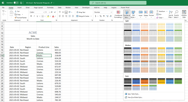
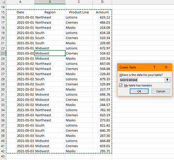
Clicking the command shows the Table formats available. Select the one you would like to use. Now confirm the range chosen by Excel is correct and that it has identified your first row has headers.
The range of related cells is now an Excel Table. Note the Table Design tab at the end of the ribbon. This tab is only available when you have selected a cell within the Table. The tab provides access to the Excel Table tools, including the place to change the table name, which I recommend doing.
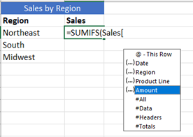
To demonstrate one of the significant advantages of Excel Tables, we will summarize the data using the sumifs function. The sumifs function sums a range of cells based on up to 127 different criteria.
The sum range in the formula is the table name plus the column header in square brackets sales[Amount]. When typing the formula, the autocomplete will show the table name in the list of options. Then after entering the opening “[“ the list of headers is displayed in the autocomplete for selection.
If you would like to bring your Excel skills to a new level with Excel Tables, please check out our webinar K2’s Excel Tables – Database Technology Comes to Spreadsheets – On Demand (2 hours)
Enjoy Excel Tables within your workbooks.


 RSS Feed