How to Format Excel PivotTables for Even Greater Effect

One of the unfortunate misconceptions regarding PivotTables in Excel is that you cannot format them to meet your specific reporting needs. Of course, the reality is that you can apply formats to your PivotTables to, in most cases, meet your exacting specifications. Read on, and in this article, you will learn just how easy it is to format your PivotTables for even greater effect.

Default Formatting in PivotTables

To begin, consider the excerpt of the PivotTable pictured in Figure 1. This raw report, although computationally correct, is difficult to read. For example, the Compact format makes the data in the first column challenging to follow.

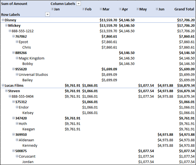
Figure 1 - Excerpt of Unformatted PivotTable

Fortunately, you can change the layout of the report quickly. To do so, click Report Layout from the PivotTable Design tab of the Ribbon. Then choose Show in Tabular Form to change the report’s appearance to that pictured in Figure 2. In this layout, notice that the entries that were “nested” in column A previously now occupy individual columns, so they report appears less cluttered.

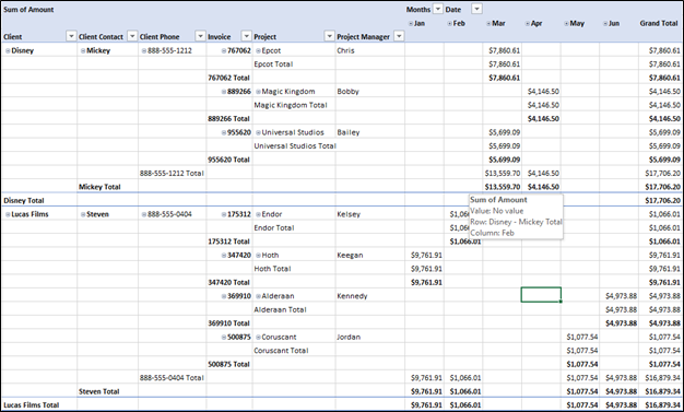
Figure 2 - PivotTable Which Uses The Tabular Layout

If you run Excel 2016 or newer, you can make the Tabular Form your default layout for all future PivotTables you create. To do so, click File, Options, Data, Edit Default Layout, as shown in Figure 3. Additionally, notice that you can make changes to other default settings for your PivotTables in that dialog box.

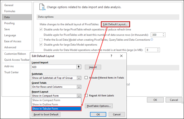
Figure 3 - Changing Default Settings For Future PivotTables

Disable Unnecessary Subtotals

In addition to the formatting changes outlined above, you may want to disable unnecessary subtotals in the body of the PivotTable. Often, subtotals contribute to a “cluttered” appearance of the data. To disable Subtotals, click on the PivotTable, and then click Subtotals, Do Not Show Subtotals on the PivotTable Design tab of the Ribbon. Upon doing so, the PivotTable will suppress Subtotals in the body of the report, as shown in Figure 4.

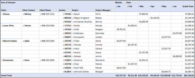
Figure 4 - PivotTable Without Subtotals

Repeat Item Labels in the PivotTable

In addition to the previous two customizations, consider repeating all the item labels in your PivotTable. This feature is especially helpful if you also choose to “collapse” the PivotTable, as discussed below.

To turn on the Repeat All Item Labels, again return to the PivotTable Design tab of the Ribbon. Then click Report Layout, followed by Repeat All Item Labels. As Figure 5 shows, this action fills the data in the Client, Client Contact, and Client Phone fields of the PivotTable, creating a format that many will find familiar.

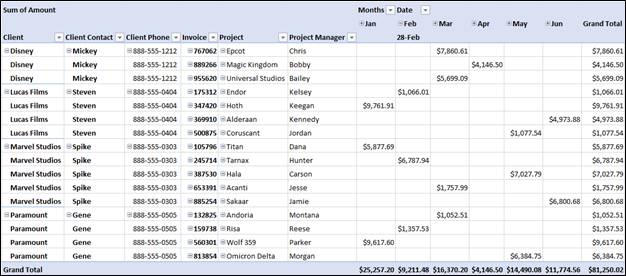
Figure 5 - Repeat Item Labels In A PivotTable

Consider Using the Collapse Field Option

If your PivotTable report is particularly lengthy, you may also want to activate the Collapse Field option. Doing so will present a summarized PivotTable with the capability of drilling-in to the report for more details. In this illustration, let us “collapse” the data in the Client column of the summary. To do so, click anywhere in that column in the PivotTable and then choose Collapse Field from the PivotTable Analyze tab of the Ribbon. After doing so, you will be able to drill in on the report to see details, without being overwhelmed by all the data contained in the summarization.  

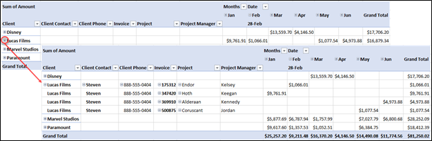
Figure 6 - Using The Collapse Field Option

Summary

No doubt, you can take advantage of other formatting options in PivotTables, including font, font size, colors, and others. However, most users do not struggle with applying those formats. On the other hand, many Excel users labor to control the volume of data presented in their reports. These same users also often face challenges with making the data easier to read. Addressing the four items outlined in this article – 1) establishing default formatting, 2) disabling unnecessary subtotals, 3) repeating item labels, and 4) using the collapse field option – you can quickly and easily format PivotTables for even greater effect.

You can learn more about PivotTables by participating in K2's Excel PivotTables for Accountants.
Also, you can learn more about establishing default settings for your PivotTables by clicking here.

You can see this tip in action by watching the video below.

Tommy Stephens