Rethinking Sorting and Filtering in Excel

New Functions Provide Superior Options!

When sorting or filtering data in Excel, most users instinctively click the drop-down arrows at the top of a column to initiate the process.  Alternatively, they flock to the Data tab of the Ribbon and click on the Sort or Filter icons there. While there is certainly nothing wrong with either of these approaches, better options exist if you are using Excel provided through a Microsoft 365 or Office 365 subscription. In this tip, you will learn how to take advantage of these better options, namely Excel’s SORT and FILTER functions.

Origins of Excel's SORT and FILTER Functions

For Microsoft 365 and Office 365 subscribers, the SORT and FILTER functions first appeared in the 1907 release of Excel (July 2019.) Neither of these functions is available in Excel 2019 or prior. Assuming you have access to Excel provided through an Office 365 subscription, you should have access to both SORT and FILTER, along with several other functions that create dynamic arrays.

Dynamic arrays are one of the most significant developments in Excel to appear in the past decade. Before dynamic arrays, we had to enter (or copy) a formula into each cell where we needed a calculation. Some refer to this as the one formula, one value paradigm. With dynamic arrays, we can enter one formula that takes action on many cells at the same time, meaning many of our Excel processes just got significantly easier!

Using Excel's SORT and FILTER Functions

Excel’s SORT and FILTER functions are relatively simple and easy to use. The syntax for the SORT function appears below.

=SORT(Array, Sort_index, Sort_order, By_col)

The array is the range of data you want to sort. The sort_index is the column by which you want to sort the array. By default, the sort_index is the first column, but you can enter a numerical reference to any other column. The sort_order defaults to a value of “1,” representing ascending; you can change this to “-1” to sort in descending order. Finally, the by_col reference defaults to False to facilitate sorting by row. If you need to sort by column instead, change the value to True.

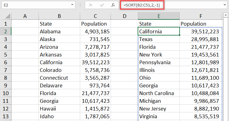
To illustrate working with the SORT function, consider the example presented in Figure 1. The SORT function used sorts the data in cells B2 through C51 on the second column (population), and it sorts the data in descending order. Notice that the formula places the results into E2 through F51. The procedure does not alter the source data range (B2 through C51) at all.

Figure 1 - Using Excel's SORT Function

Working With the Filter Function

Excel’s FILTER function is similar to SORT is some regards, but its fundamental purpose is decidedly different. That is, you can use FILTER to reduce the volume of data to only those rows that meet specific criteria. The syntax for FILTER appears below.

=FILTER(Array, Include, if_empty)

Like SORT, when using FILTER, the array argument is the range you wish to screen to meet specific criteria. The include argument allows you to specify your screening criteria.  Finally, you can use if_empty to indicate what gets returned if no records match the specified criteria.

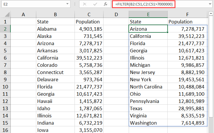
Figure 2 illustrates working with the FILTER function in Excel. In this example, the formula filters the data in cells B2 through C51 to just those states with populations exceeding 7,000,000. Like the SORT function, the FILTER function does not disturb or otherwise rearrange the source data.

Figure 2 - Working with Excel's Filter Function

Notably, you can “nest” SORT and FILTER in the same formula for even better reporting and analyses. For example, the formula shown below filters the data first and then sorts the records that match the filter criteria.

=SORT(FILTER(E2:F51,F2:F51>7000000),2,-1)

Summary

Both SORT and FILTER are available to many Excel users, yet most remain unaware of their presence and, therefore, do not take advantage of these functions. Both these functions facilitate quicker and more robust analyses of data. They also allow you to take action on a range or table of data without affecting the data in that range or table. Further, they do not disturb or rearrange the source data, and you can nest them in the same formula for even more power. In sum, if you have access to SORT and FILTER, consider how you can use them to improve your reporting processes. If you don’t yet have access to these functions, stay alert for when they do become available to you so that you can take advantage of them at that time.

Tommy Stephens