
As you are no doubt aware, Microsoft added many new features with the release of Excel 2019. Further, the tech giant continues to update the venerable spreadsheet application through updates to Office 365. Of course, these new features do not pay dividends unless you are aware of them and know how to put them to use. Read on, and in this article, you will learn about five of the most significant new features in Excel and how you can take advantage of them.
Automate Data Analysis with Excel’s Ideas Feature
Ideas is a form of artificial intelligence incorporated into Excel available through Office 365 subscriptions. With Ideas, Excel can analyze your data quickly and provide you with insights that you may not have noticed otherwise. For example, Ideas could be useful in the following situations:
If you run Excel through an Office 365 subscription, you can access Ideas from the Home tab of the Ribbon. Note, however, that you must have an active internet connection to use this feature.
- Analyzing transactions to rank data and identify items(s) that are significantly larger or smaller than the rest of the population;
- Performing trend analysis to highlight trends over data based on the passage of time;
- Identifying significant outliers in data points, including potentially erroneous or fraudulent transactions; and
- Calling attention to situations where a substantial portion of the total value is attributable to a single factor.
If you run Excel through an Office 365 subscription, you can access Ideas from the Home tab of the Ribbon. Note, however, that you must have an active internet connection to use this feature.
Simpler Conditional Formulas with IFS, MAXIFS, and MINIFS
With IFS, MAXIFS, and MINIFS , you can create formulas that contain multiple tests more easily than in the past. Before the availability of IFS, many Excel users often “nested” multiple IF functions in the same formula. This was a common practice when needing to create a calculation based on satisfying one or more conditions. However, with the introduction of IFS, such formulas are simplified greatly. For example, notice in the formula below that only one IFS function is required to perform three tests of the data in cell A2. This technique contrasts with multiple IF functions that would have been required in the past.
=IFS(A2>400,”Tier 1″,A2>300,”Tier 2″,TRUE,”Tier 3″)
Like IFS, you can use MAXIFS and MINIFS to perform multiple tests of your data. When using MAXIFS, Excel will return the largest value when all the tests are satisfied. Conversely, when using MINIFS, Excel will return the smallest value when all the tests are satisfied.These functions are available to Excel 2019 users. Also, they are available to users of Excel provided through Office 365 subscriptions.
XLOOKUP – A Better and Easier Alternative to VLOOKUP
Microsoft added XLOOKUP to Excel provided through Office 365 beginning in February 2020. XLOOKUP offers a superior alternative to VLOOKUP and similar functions such as HLOOKUP and INDEX. While these legacy functions will remain in Excel, many users will find XLOOKUP to be more straightforward and intuitive. Most will also find XLOOKUP to be even more powerful. Some of the critical differences between XLOOKUP and other lookup functions include:
- XLOOKUP defaults to an exact match, whereas VLOOKUP and HLOOKUP default to an approximate match.
- With XLOOKUP, you do not have to specify a column index number as you do with VLOOKUP or a row index number as you do with HLOOKUP.
- The arrangement of columns and rows does not matter with XLOOKUP. This is because the function can look to the left or right when using it as an alternative to VLOOKUP. Likewise, it can look above or below when using it as an alternative to HLOOKUP.
- XLOOKUP allows you to specify what happens if your lookup value isn’t found, without having to include an IFERROR function.
Illustrating XLOOKUP
To begin to understand the advantages of working with XLOOKUP, consider the example presented in Figure 1. In this illustration, XLOOKUP is used to find the value from cell H2 in the range of B3 through B15. Keep in mind, XLOOKUP defaults to an exact match, whereas VLOOKUP defaults to an approximate match. Once it finds the value it is looking for, XLOOKUP returns the corresponding value from the range D3 through D15. If no match is found, then the formula would return the phrase “Item Not Found.” Because of the relative simplicity of XLOOKUP compared to VLOOKUP, HLOOKUP, and other similar functions, XLOOKUP likely will become the preferred lookup function as more users gain access to it.
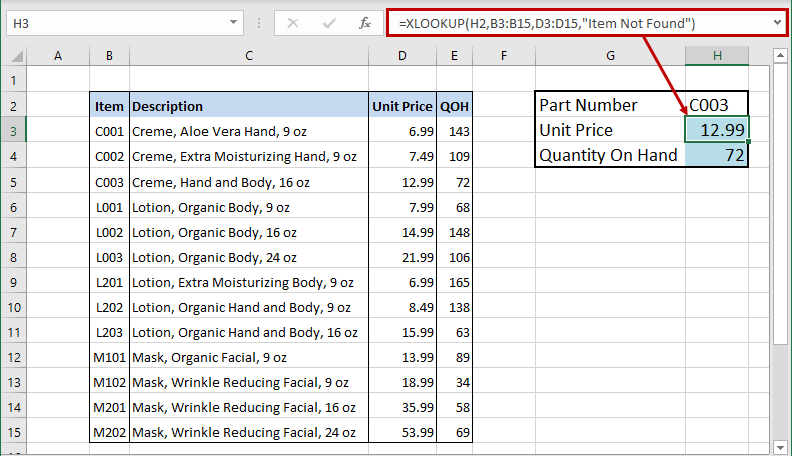
Figure 1 - Using XLOOKUP Instead of VLOOKUP
Dynamic Arrays
Dynamic arrays are another example of a new feature that is currently available only through an Office 365 subscription. With dynamic arrays, you can write a single formula that acts on multiple cells simultaneously, without having to copy the formula to all the cells. Additionally, if you are running a version of Excel that supports dynamic arrays, you no longer need to use a CTRL + SHIFT + ENTER keystroke sequence to enter a traditional array formula. Further, if you are using a version of Excel that supports dynamic arrays, six new functions are available to you to help you capitalize on this new-found power. These six functions include FILTER, SORT, RANDARRY, SEQUENCE, SORTBY, and UNIQUE.
Illustrating Dynamic Arrays
Let us demonstrate a simple example of dynamic arrays by using the new FILTER function. As implied by its name, the FILTER function is capable of filtering data in a table or a range via a formula. The syntax is relatively simple, as shown below.
=FILTER(array (table or range), include (a Boolean array for which items to include))
An optional third argument – [if_empty] – specifies the value to display if the filter returns nothing. Figure 2 below displays an example of how you can use the FILTER function to filter data without disturbing the original array. Notably, if the volume of data in the table referenced by the FILTER function increases or decreases, so too will the volume of the data returned by the formula.
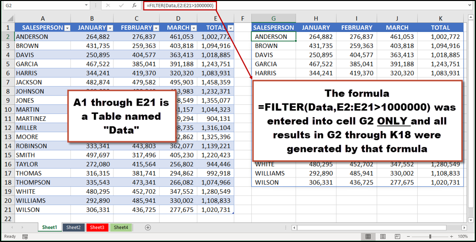
Figure 2 - Using FILTER to Create a Dynamic Array
The simple FILTER example provided should begin to highlight the power of dynamic arrays – they allow you to use formulas to analyze data, and the formula results are linked to but do not disturb the original data set. Therefore, you can perform multiple types of analyses on the same underlying data set, without having to copy the data multiple times.
Analyze the Quality of Your Data with Power Query
First available with the 2010 release of Excel, the evolution of Power Query is nothing short of remarkable. You can use this utility to query data into Excel from countless external data sources, including the databases supporting most major accounting applications. Perhaps more importantly, you can use Power Query to transform your data to make it more useful to you. These transformations, for example, could include items such as deleting unnecessary columns of data, merging columns, adding user-defined calculations, and sorting and filtering as part of the query, among other items.
A recent enhancement to Power Query is its’ ability to automatically analyze your data for quality issues such as completeness and accuracy. With this feature, you can quickly identify potential problem areas such as erroneous data, missing records, and even duplicated records. To take advantage of this feature, on the View tab of the Power Query Editor, check the Column quality, Column distribution, and Column profile boxes, as shown in Figure 3. As you can see, Power Query generates a “quality snapshot” of each of the columns of data in the query; further, clicking on any column in the query exposes a more detailed view of the data, including statistics for that column and a value distribution graph. This feature was made available beginning in February 2020 for Office 365 subscribers.
A recent enhancement to Power Query is its’ ability to automatically analyze your data for quality issues such as completeness and accuracy. With this feature, you can quickly identify potential problem areas such as erroneous data, missing records, and even duplicated records. To take advantage of this feature, on the View tab of the Power Query Editor, check the Column quality, Column distribution, and Column profile boxes, as shown in Figure 3. As you can see, Power Query generates a “quality snapshot” of each of the columns of data in the query; further, clicking on any column in the query exposes a more detailed view of the data, including statistics for that column and a value distribution graph. This feature was made available beginning in February 2020 for Office 365 subscribers.
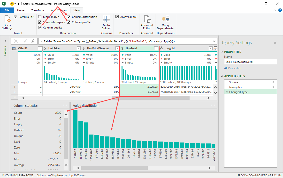
Figure 3 - Using Power Query to Analyze Data Quality
Summary
By no means do the five features listed above represent all the new features available in Excel. On the contrary, Microsoft has added over a hundred new features and enhancements to Excel over the past five years! Instead, the tools outlined in this article are among those that offer some of the greatest opportunities to all levels of Excel users to improve their efficiency and proficiency. Therefore, as you gain access to these tools – and others sure to follow – be sure to consider how you and your team members can and should take advantage of them to boost productivity.
 RSS Feed